Bachelor of Ecole Polytechnique MAA106: Introduction to Numerical Analysis, year 1, semester 2 Maxime Breden
Based on Notebooks created by Aline Lefebvre-Lepot

Introduction to Numpy and Matplotlib (Correction)

 

                

This tutorial gives a quick overview on how to use the python packages Numpy and Matplotlib.

Table of contents

• Numpy
• Matplotlib

Numpy

NumPy is the fundamental package for scientific computing with Python (see http://www.numpy.org/). It contains powerful N-dimensional array objects, linear algebra, Fourier transform, random numbers and also sophisticated tools for integrating C++ and Fortran code.

In this class, we are going to use this package essentially to manipulate arrays. Lot of documentations about numpy can be found on the web, we give below basic examples that will be useful in the following.

First, you need to import the numpy package:

import numpy as np

Creating arrays

# One-dimensional arrays
a = np.array([0, 1, 2, 3])
print('a =',a)
print('a.shape =', a.shape)
print('a.size =', a.size)

a = [0 1 2 3]
a.shape = (4,)
a.size = 4

# Two-dimensional arrays
R1 = [0, 1, 2, 3]
R2 = [4, 5, 6, 7]
a = np.array([R1, R2])
print('a =', a)
print('a.shape =', a.shape)
print('a.size =', a.size)

a = [[0 1 2 3]
 [4 5 6 7]]
a.shape = (2, 4)
a.size = 8

You can use tabulation in notebooks for autocompletion or to obtain the list of possible completions. You can also obtain interactive help:

np.array?

There exists several functions to create arrays:

# imposing the number of elements
c = np.linspace(0, 1, 6)   # start, end, number of points
print('c =', c)

c = [0.  0.2 0.4 0.6 0.8 1. ]

# imposing the step between the elements
a = np.arange(10) # 0 .. n-1  (!) start=0 and step=1 by default
b = np.arange(1, 9, 2) # start, end (exclusive), step
c = np.arange(1, 2, 0.1) # start, end (exclusive), step
print('a =', a)
print('b =', b)
print('c =', c)

a = [0 1 2 3 4 5 6 7 8 9]
b = [1 3 5 7]
c = [1.  1.1 1.2 1.3 1.4 1.5 1.6 1.7 1.8 1.9]

# arrays of 0's or 1's with given size
a = np.zeros(2) # 1 dimensional, number of elements
b = np.ones(3) # 1 dimensional, number of elements
c = np.zeros((2, 3)) # 2-dimensional, tuple (number of rows, number of columns)
print('a =', a)
print('b =', b)
print('c =', c)

a = [0. 0.]
b = [1. 1. 1.]
c = [[0. 0. 0.]
 [0. 0. 0.]]

# random initialization
a = np.random.rand(4) # uniform in [0,1]
b = np.random.randn(4) # gaussian
print('a =', a)
print('b =', b)

a = [0.36535976 0.96249138 0.77985216 0.31913144]
b = [ 1.20131701  2.03115812 -0.65134299  0.71157022]

• Create a null vector of size 10.
• Create a vector with values ranging from 10 to 49.
• create a vector with values ranging from 0 to 1 with 100 points.
• Create a 3x3 random matrix.
• Print the shape of the previous arrays.

a = np.zeros(10)
print("a =",a,", shape :",a.shape)

a = np.arange(10,50)
print("\na =",a,", shape :",a.shape)

a = np.linspace(0,1,100)
print("\na =",a,", shape :",a.shape)

a = np.random.random((3,3))
print("\na =",a,", shape :",a.shape)

a = [0. 0. 0. 0. 0. 0. 0. 0. 0. 0.] , shape : (10,)

a = [10 11 12 13 14 15 16 17 18 19 20 21 22 23 24 25 26 27 28 29 30 31 32 33
 34 35 36 37 38 39 40 41 42 43 44 45 46 47 48 49] , shape : (40,)

a = [0.         0.01010101 0.02020202 0.03030303 0.04040404 0.05050505
 0.06060606 0.07070707 0.08080808 0.09090909 0.1010101  0.11111111
 0.12121212 0.13131313 0.14141414 0.15151515 0.16161616 0.17171717
 0.18181818 0.19191919 0.2020202  0.21212121 0.22222222 0.23232323
 0.24242424 0.25252525 0.26262626 0.27272727 0.28282828 0.29292929
 0.3030303  0.31313131 0.32323232 0.33333333 0.34343434 0.35353535
 0.36363636 0.37373737 0.38383838 0.39393939 0.4040404  0.41414141
 0.42424242 0.43434343 0.44444444 0.45454545 0.46464646 0.47474747
 0.48484848 0.49494949 0.50505051 0.51515152 0.52525253 0.53535354
 0.54545455 0.55555556 0.56565657 0.57575758 0.58585859 0.5959596
 0.60606061 0.61616162 0.62626263 0.63636364 0.64646465 0.65656566
 0.66666667 0.67676768 0.68686869 0.6969697  0.70707071 0.71717172
 0.72727273 0.73737374 0.74747475 0.75757576 0.76767677 0.77777778
 0.78787879 0.7979798  0.80808081 0.81818182 0.82828283 0.83838384
 0.84848485 0.85858586 0.86868687 0.87878788 0.88888889 0.8989899
 0.90909091 0.91919192 0.92929293 0.93939394 0.94949495 0.95959596
 0.96969697 0.97979798 0.98989899 1.        ] , shape : (100,)

a = [[0.63519514 0.66440185 0.69371797]
 [0.9009795  0.8778431  0.85348441]
 [0.63015241 0.19813284 0.74811969]] , shape : (3, 3)

Indexing of arrays

The elements are indexed from 0:

• the first element has index 0
• the second element has index 1 etc...

The elements can also been indexed from the end:

• the last element can be obtained using index -1
• the second to last can be obtained using index -2 etc...

# One dimensional arrays
a = np.arange(8)
print('a =', a)
print('elements =', a[0], a[4], a[-1], a[-3])  # extract an elements, 0 = first, 1 = second..., -1 = last

a = [0 1 2 3 4 5 6 7]
elements = 0 4 7 5

# Two dimensional arrays
R1 = [0, 1, 2, 3, 4, 5]
R2 = [10, 11, 12, 13, 14, 15]
a = np.array([R1, R2])
print(a)
print('element =', a[1, 3]) # extract an element, 0 = beginning, -1 = end (2nd row, 4th column) 
print('column =', a[:, 2]) # extract a column, 0 = beginning, -1 = end
print('row =', a[1, :]) # extract a row, 0 = beginning, -1 = end

[[ 0  1  2  3  4  5]
 [10 11 12 13 14 15]]
element = 13
column = [ 2 12]
row = [10 11 12 13 14 15]

Slicing of arrays

Slicing of arrays is based on the following indexing where [: is the default start and :] the default end. Except if using the default end, the last element is excluded from the selection.

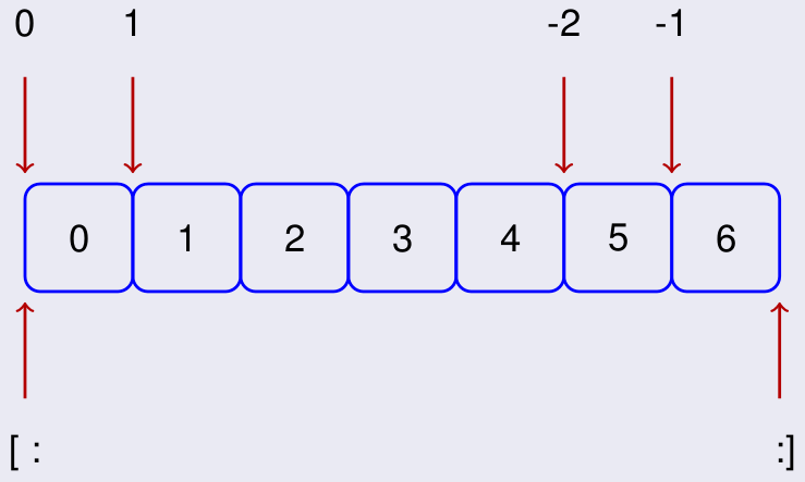
It is a powerful way of extracting sub-arrays from a given array.

• Successively uncomment the various extractions of the array a defined in the following cell, by using "ctrl+/" or by deleting the "#" symbol at the beginning of each line, to see how slicing works in practice.

## Slicing one dimensional arrays
a = np.arange(10)
print('a =', a)
print('extract 1 =', a[1:7:2])   # start, end (exclusive), step
print('extract 2 =', a[1:7:])    # default step = 1
print('extract 3 =', a[:7:2])    # default start = first element (= 0)
print('extract 4 =', a[3::1])    # default end = until last element 
print('extract 5 =', a[3:-1:1])  # !!! if end = -1, the last element is excluded (see figure)
print('extract 6 =', a[6:2:-1])  # negative step

## short commands:
print('extract 7 =', a[1:7])     # same result as extract 2: default step=1
print('extract 8 =', a[3:])      # same result as extract 4: default step=1, default end=last element
print('extract 9 =', a[:3])      # default step=1, default start=1st element

a = [0 1 2 3 4 5 6 7 8 9]
extract 1 = [1 3 5]
extract 2 = [1 2 3 4 5 6]
extract 3 = [0 2 4 6]
extract 4 = [3 4 5 6 7 8 9]
extract 5 = [3 4 5 6 7 8]
extract 6 = [6 5 4 3]
extract 7 = [1 2 3 4 5 6]
extract 8 = [3 4 5 6 7 8 9]
extract 9 = [0 1 2]

# Slicing two dimensional arrays
R1 = [0, 1, 2, 3, 4, 5]
R2 = [10, 11, 12, 13, 14, 15]
a = np.array([R1, R2])
print('a =', a)
print('extract =', a[0, ::2])

a = [[ 0  1  2  3  4  5]
 [10 11 12 13 14 15]]
extract = [0 2 4]

# slicing can also be used to assign values in an array
a = np.zeros(10)
a[::2] = 1
print('a =', a)

a = [1. 0. 1. 0. 1. 0. 1. 0. 1. 0.]

• Create a 2-d array of size 10x10, with 1's on the borders and 0's inside.

Z = np.ones((10,10))
Z[1:-1,1:-1] = 0
print(Z)

[[1. 1. 1. 1. 1. 1. 1. 1. 1. 1.]
 [1. 0. 0. 0. 0. 0. 0. 0. 0. 1.]
 [1. 0. 0. 0. 0. 0. 0. 0. 0. 1.]
 [1. 0. 0. 0. 0. 0. 0. 0. 0. 1.]
 [1. 0. 0. 0. 0. 0. 0. 0. 0. 1.]
 [1. 0. 0. 0. 0. 0. 0. 0. 0. 1.]
 [1. 0. 0. 0. 0. 0. 0. 0. 0. 1.]
 [1. 0. 0. 0. 0. 0. 0. 0. 0. 1.]
 [1. 0. 0. 0. 0. 0. 0. 0. 0. 1.]
 [1. 1. 1. 1. 1. 1. 1. 1. 1. 1.]]

• Create a 8x8 matrix and fill it with a checkerboard pattern of 0's and 1's.

Z = np.zeros((8,8),dtype=int)
Z[1::2,::2] = 1 # even rows: 2-4-6-8
#print(Z)
Z[::2,1::2] = 1 # odd rows: 1-3-5-7
print(Z)

[[0 1 0 1 0 1 0 1]
 [1 0 1 0 1 0 1 0]
 [0 1 0 1 0 1 0 1]
 [1 0 1 0 1 0 1 0]
 [0 1 0 1 0 1 0 1]
 [1 0 1 0 1 0 1 0]
 [0 1 0 1 0 1 0 1]
 [1 0 1 0 1 0 1 0]]

• Create a random vector of size 5 and exchange the maximal and minimal values

v = np.random.random(5)
print(v)
vmax = np.max(v)
imax = np.argmax(v)
vmin = np.min(v)
imin = np.argmin(v)
v[imax] = vmin
v[imin] = vmax
print(v)

[0.30685449 0.3270097  0.68052487 0.02125102 0.33021165]
[0.30685449 0.3270097  0.02125102 0.68052487 0.33021165]

Loops and computations on arrays

• Save your notebook...

Loop counters are designed so that one can scan an array using a.shape:

a = np.zeros((2, 3)) 
for i in range(a.shape[0]):
    for j in range(a.shape[1]):
        a[i, j] = (i + 1)*(j + 1)
print('a =', a)

a = [[1. 2. 3.]
 [2. 4. 6.]]

However, numpy has built-in element-wise array operations, and one should typically avoid using loops on arrays when possible.

a = np.linspace(0, 1, 1000000)
b = np.zeros(1000000)
for i in range(a.size): b[i] = 3*a[i] - 1
print("Done")

Done

a = np.linspace(0, 1, 1000000)
b = 3*a - 1
print("Done")

Done

# b = 3a-1 with a loop
a = np.linspace(0, 1, 1000000)
b = np.zeros(1000000)
%timeit for i in range(a.size): b[i] = 3*a[i] - 1

309 ms ± 3.15 ms per loop (mean ± std. dev. of 7 runs, 1 loop each)

# b = 3a-1 with arrays
a = np.linspace(0, 1, 1000000)
%timeit b = 3*a - 1

815 µs ± 44.9 µs per loop (mean ± std. dev. of 7 runs, 1,000 loops each)

Numpy also provides various optimized functions as sin, exp... for arrays

def f(x):
    return np.exp(-x*x)*np.log(1 + x*np.sin(x))

print("test 1")
x = np.linspace(0, 1, 100000)
a = np.zeros(x.size)
%timeit for i in range(x.size): a[i] = f(x[i])

print("test 2")
x = np.linspace(0, 1, 100000)
%timeit a = f(x)

test 1
191 ms ± 1.28 ms per loop (mean ± std. dev. of 7 runs, 10 loops each)
test 2
937 µs ± 42.2 µs per loop (mean ± std. dev. of 7 runs, 1,000 loops each)

• Save your notebook...
• Create two random vectors $x$ and $y$ of size $n=10$.
• Assuming $x$ and $y$ represent the cartesian coordinates of 10 points $(x_k,y_k)$, compute two new vectors $r$ and $\theta$ representing the polar coordinates of these points.
• Optimize and test your code for vectors $x$ and $y$ of size $n=10^5$ (compare efficiency of a loop, list comprehension and numpy element-wise operations on arrays).

n = 10
x = np.random.random(n)
y = np.random.random(n)
r = np.sqrt(x**2+y**2)
theta = np.arctan2(y,x)
print(r)
print(theta)

[0.39457698 0.6797513  0.98444721 0.96527823 0.88184501 1.05834794
 0.66450096 0.11760212 1.11431188 0.78296806]
[0.2976864  0.62613259 0.36289393 1.09500816 1.14617758 0.36140722
 0.1031102  0.32434819 0.58153296 0.90146435]

The above answer is the "cleanest one", but it requires you to know about the function numpy.arctan2, which automatically handles the degenerate cases (when $x=0$). It is also possible to only use the function numpy.arctan, and for this specific example it doesn't matter much because the probability of having and $x_k$ equal to $0$ is almost zero, but in principle one should also make sure that these singular cases are properly handled.

# optimized version: use numpy vectors
n = 10**5
x = np.random.random(n)
y = np.random.random(n)
%timeit r = np.sqrt(x**2+y**2)
%timeit theta = np.arctan2(y,x)

84.5 µs ± 443 ns per loop (mean ± std. dev. of 7 runs, 10,000 loops each)
2.21 ms ± 17.4 µs per loop (mean ± std. dev. of 7 runs, 100 loops each)

# non optimized version: for loop
n = 10**5
x = np.random.random(n)
y = np.random.random(n)
r = np.zeros(n)
theta = np.zeros(n)
from math import sqrt, atan2
%timeit for i in range(n): r[i] = sqrt(x[i]**2+y[i]**2)
%timeit for i in range(n): theta[i] = atan2(y[i],x[i])

46.5 ms ± 473 µs per loop (mean ± std. dev. of 7 runs, 10 loops each)
20.7 ms ± 323 µs per loop (mean ± std. dev. of 7 runs, 10 loops each)

# barely faster than a for loop: list comprehension
n = 10**5
x = np.random.random(n)
y = np.random.random(n)
%timeit r = [sqrt(x[i]**2+y[i]**2) for i in range(n)]
%timeit theta = [atan2(y[i],x[i]) for i in range(n)]

42.6 ms ± 291 µs per loop (mean ± std. dev. of 7 runs, 10 loops each)
17.4 ms ± 798 µs per loop (mean ± std. dev. of 7 runs, 100 loops each)

Matplotlib

Matplotlib is a Python package for 2 dimensional plots. It can be used to produce figures inline in jupyter notebooks. Lots of documentation about matplotlib can be found on the web, we give below basic examples that will be useful for the rest of the course.

First, we need to import the matplotlib package.

# In order to display plots inline:
%matplotlib inline   

# load the libraries
import matplotlib.pyplot as plt # 2D plotting library
import numpy as np              # package for scientific computing  
plt.rcParams["font.family"] ='Comic Sans MS'

First plot

We plot on the same figure sine and cosine on the interval $[-\pi, \pi]$.

X = np.linspace(-np.pi, np.pi, 30)
COS, SIN = np.cos(X), np.sin(X)
plt.plot(X,COS)
plt.plot(X, SIN)
plt.show()

Modifying properties of the figure

Most of the properties of a figure can be customized: color and style of the graphs, title, legend, labels... Below, we plot on the same figure with sine and cosine on the interval $[-\pi, \pi]$, specifying some of the properties of the figure. You can try to comment or modify these properties...

# creates a figure with size 10x5 inches
fig = plt.figure(figsize=(10, 5))

# plot cosine, blue continuous line, width=5, label=cosine
plt.plot(X, COS, color="blue", linestyle="-", linewidth=5, label='cosine')

# plot sine, red dotted line, width=1, label=sine
plt.plot(X, SIN, color="red", linestyle="--", linewidth=1, label='sine')

# specify x and y limits
plt.xlim(-np.pi*1.1, np.pi*1.1)
plt.ylim(-1.1, 1.1)

# add a label on x-axis
plt.xlabel('x', fontsize=18)

# add a title
plt.title('Cosine and Sine functions', fontsize=18)

# add a legend located at the top-left of the figure
plt.legend(loc='upper left', fontsize=16)

# show the figure
plt.show()

• On the same figure, plot $x\to 1-\cos(x)$ and $x\to x-\sin(x)$ for $x\in [0,\pi]$.
• Add a legend.
• On another figure, plot the same functions using a loglog scale (use plt.loglog, to plot log(f(x)) versus log(x)).

from math import pi
x = np.linspace(0,pi,1000)
f = 1 - np.cos(x)
g = x - np.sin(x)

fig = plt.figure(figsize=(10, 5))
plt.plot(x,f,label="f(x) = 1 - cos(x)")
plt.plot(x,g,label="g(x) = x - sin(x)")
plt.xlabel('x')
plt.legend(fontsize=16)
plt.show()

x = np.linspace(0,pi,1000)
f = 1 - np.cos(x)
g = x - np.sin(x)

fig = plt.figure(figsize=(10, 5))
plt.loglog(x,f,label="f(x) = 1 - cos(x)")
plt.loglog(x,g,label="g(x) = x - sin(x)")
plt.xlabel('x')
plt.loglog(x,x**2,'k--',label="slope 2")
plt.loglog(x,x**3,'k:',label="slope 3")
plt.legend(fontsize=16)
plt.show()

• What do you notice on the loglog plot? Can you explain it? Create a text-cell with style "Answer" to write your comments.

The curves seem almost straight in this scale. Indeed, we have $f(x) \approx x^2/2$ and $g(x)\approx x^3/6$ when $x$ goes to zero. Therefore $\ln f(x) \approx 2\ln x - \ln 2$ and $\ln g(x)\approx 3\ln x -\ln 6$, and we expect the two curves to be close to lines having slope $2$ and $3$ respectively. We observe on the picture that the slopes are the expected ones.

Creating several subfigures

A “figure” in matplotlib means the whole window in the user interface. Within this figure there can be “subplots”. In the following, we use subplots to draw sine and cosine in two different plots.

# create the figure
fig = plt.figure(figsize=(10, 5))

# Create a new subplot 
# input: (num-lines, num-columns, num of the current plot)
plt.subplot(1, 2, 1)  # grid 1 x 2, current plot =1
plt.plot(X, COS, color="blue", linestyle="-", linewidth=1)
plt.xlim(-np.pi*1.1, np.pi*1.1)
plt.ylim(-1.1, 1.1)
plt.title('Cosine function', fontsize=18)

# Create a new subplot 
plt.subplot(1, 2, 2)  # grid 1 x 2, current plot = 2
plt.plot(X, SIN, color="red", linestyle="-", linewidth=1)
plt.xlim(-np.pi*1.1, np.pi*1.1)
plt.ylim(-1.1, 1.1)
plt.title('Sine function', fontsize=18)

plt.show()

Using equal axes

It is also possible to impose the same scale on both axes. As an example, we plot below a circle of radius 1:

# create the figure
fig = plt.figure(figsize=(15, 5))

# Create a new subplot 
plt.subplot(1, 2, 1)  # grid 1 x 2, current plot =1
plt.plot(COS, SIN, color="blue", linestyle="-", linewidth=1)
plt.title('Without equal axes', fontsize=18)

# Create a new subplot 
plt.subplot(1, 2, 2)  # grid 1 x 2, current plot = 2
plt.axis('equal')
plt.plot(COS, SIN, color="red", linestyle="-", linewidth=1)
plt.title('With equal axes', fontsize=18)

plt.show()

• Plot the butterfly curve.

t = np.linspace(0,12*pi,1000)
x = np.sin(t) * (np.exp(np.cos(t)) - 2* np.cos(4*t) - np.sin(t/12)**5)
y = np.cos(t) * (np.exp(np.cos(t)) - 2* np.cos(4*t) - np.sin(t/12)**5)

plt.figure()
plt.plot(x,y)
plt.axis('equal')
plt.title("The butterfly curve!")
plt.show()

To go further...

Lots of documentation and tutorials can be found on the web about Numpy and Matplotlib. A very complete tutorial for scientific python can be found here http://www.scipy-lectures.org/index.html. In particular, you can have a look at the two following chapters:

• Numpy: http://www.scipy-lectures.org/intro/numpy/index.html
• Matplotlib: http://www.scipy-lectures.org/intro/matplotlib/index.html

# execute this part to modify the css style
from IPython.core.display import HTML
def css_styling():
    styles = open("../style/custom3.css").read()
    return HTML(styles)
css_styling()